Dynamic Algebra: Plot a Function and its Family

A Sketchpad coordinate system has two axes, two points, and a grid. The two points are the origin point at (0, 0) and the unit point at (1, 0).

Open a new sketch and choose Graph | Define Coordinate System.

Drag the origin point. What happens?

Drag the unit point. What happens?

Before you explore Sketchpad’s function-plotting capabilities, you’ll build a model that develops the concept of a function plot. This model starts with a point on the x-axis and its abscissa (another term for the x-coordinate).

Construct a point on the x-axis.

Drag the new point to make sure it remains on the axis. Then with the point selected, choose Measure | Abscissa (x). Drag the point—now labeled A—and observe how the measurement x_A changes.

Choose Number | Calculate to open the Calculator.

Now you’ll enter a rule that changes one value, x_A, into another. The rule in this example is to multiply by 2 and subtract 3, but you can make up your own rule if you like. (Use the ^ key to enter an exponent.)

Press the keys in the Calculator to enter an expression for your rule. For example, press the 2 key and * key, click the value x_A in your sketch, press the – key and 3 key, and click OK.

If necessary, move the Calculator when you need to click the value x_A.

Double-click the value x_A with the Text tool and change its label to In. Similarly, change the label of the new calculation to Out.

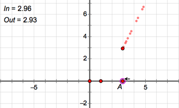
Select in order the values In and Out and choose Graph | Plot as (x, y).

Drag point A and observe how the plotted point moves.

Click in empty space to deselect all objects. Select only the plotted point and choose Display | Trace Plotted Point.

Drag point A back and forth until you can clearly see the shape formed by the traces. What do the traces represent?

Now you’ll plot a function using Sketchpad’s Calculator and explore how to change the scales of Sketchpad’s coordinate system.

Choose Graph | Plot New Function.

In the Calculator, enter the rule you used in step 7, but this time click the x key instead of the measurement in the sketch.

For example, press these keys in order: 2, *, x, –, 3, and click OK.

An equation and graph appear. If the graph does not match your traces from step 12, choose Edit | Undo and make sure you’re using the same rule.

Select point A, choose Edit | Cut (or press the Delete key), and choose Display | Erase Traces.

Double-click the function (not the plot) to open the Calculator.

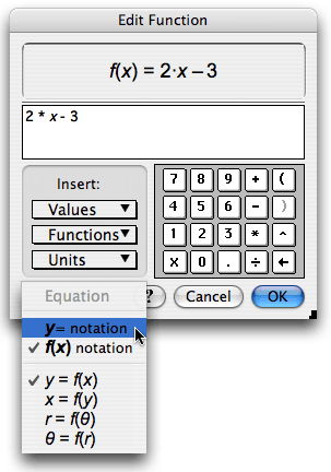
In the Calculator, choose the Equation pop-up menu and choose either f(x) notation or y= notation, depending on whether you prefer to see your function labeled f(x) = 2x – 3 or y = 2x – 3.

You can change the scales by dragging the unit point or by dragging any number along an axis. You can also use different scales on the two axes.

Drag numbers on both axes and notice how the grid changes. Center your axes and scale them so that (–10, 0) and (10, 0) are visible on the x-axis.

Choose Graph | Grid Form | Rectangular Grid. Now drag numbers on both the x-axis and the y-axis. What has changed?

Next you’ll create a parameter—a simple numeric value—and use it in to your function definition. Then you’ll explore the effect of changing the parameter.

Choose Number | New Parameter. In the dialog box, change the name to m, set its value to 2, and click OK.

Double-click the function. In the Calculator, delete the 2 in the input line, and click parameter m in the sketch to form the function f(x) = m•x – 3 (or y = m•x – 3).

Click in the parameter box and change its value to 3. What happens to the function plot?

Select the parameter and press the + key several times. Then press the – key several times. By how much does the parameter change each time? What happens to the function plot?

Select the parameter and choose Edit | Properties. On the Parameter panel, set the keyboard adjustments to change by 0.1. On the Value panel, change the precision to tenths. Then click OK.

Press the + and – keys several times and observe how the parameter and function plot change.

You can also adjust a parameter by pressing inside the edit box and dragging or flicking up or down. The parameter continues to change as long as you press.

Select the parameter and choose Display | Animate Parameter. Use the Motion Controller to pause and resume the motion, to reverse the motion, to change the speed, and finally to stop the motion.

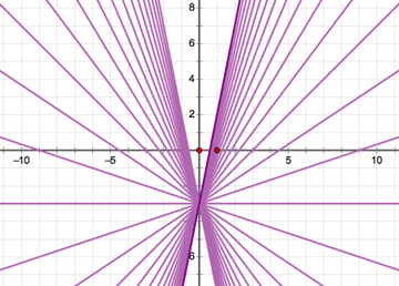
Select the graph and parameter m and choose Construct | Family of Functions. In the dialog box, specify 31 samples over a parameter domain from –10 to 10 and click OK.

What do you notice about this family of functions?

Create another parameter b with a value of –3.0 and edit the function to replace the –3 with + b. Explore the family of functions produced by varying the value of parameter b. How is this family of functions similar to or different from the last family of functions?

In a new sketch, create parameters a, b, and c and plot the function f(x) = ax² + bx + c. Experiment with changing each parameter and looking at its family of functions.

On the same page, create two more parameters, h and k, and plot the function g(x) = a(x – h)² + k. Experiment with all the parameters to explore how these two functions are similar and different.